[The peak of the Ice Age by Michael Oard]
After the Flood drained off the land, the world’s ocean and land
temperatures were constantly changing as they strove toward the relative
equilibrium we experience today. It took centuries of climate change for this to
work itself out. The warm ocean gradually cooled while the glaciers grew and
spread. The Ice Age wound down as the amount of volcanic ash and dust in the
stratosphere slowly decreased and the earth’s climates became more stable.
Finally, there came a time when the two main mechanisms of the Ice Age, volcanic
material in the stratosphere and the warm ocean, diminished so much that they
could no longer sustain a net buildup of ice over the globe. This was the peak
of the Ice Age, or glacial maximum.
Glacial maximum
As glacial maximum approached, the
ocean water and atmosphere at mid and high latitudes cooled enough for many
areas close to the ocean to glaciate (see
figures 3.8
and 3.9). The change in water and land temperatures allowed the ice sheets
to expand out onto the continental shelves off eastern Canada and New England.
Ice spread from the mountains of British Columbia and Washington State into the
surrounding lowlands. East of the Rocky Mountains, ice descended onto the high
plains and coalesced with the Laurentide ice sheet blocking the ice-free
corridor.
Ice caps, starting in the mountains of Greenland and
Scandinavia, swept down onto the lowlands. The Baltic Sea was covered with ice
by then, so ice blanketed much of northern continental Europe and northwest
Asia. About midway through the Ice Age, the British Isles developed mountain ice
caps. They would have filled in the valleys and covered the Irish Sea by the end
of the Ice Age. However, it is doubtful there was a connection between the small
ice sheet on the British Isles and the Scandinavian ice sheet across the North
Sea.
By glacial maximum the East Antarctica ice sheet in the Southern
Hemisphere had become enormous. In West Antarctica, ice descended out of the
mountains and filled up the surrounding depressions that were below sea level to
form one large West Antarctica ice sheet. The West Antarctica ice sheet merged
in places with the East Antarctica ice sheet. The mountains of South America,
New Zealand, and Tasmania were covered by ice caps. A small portion of the
mountains in southeast Australia was capped by ice.
In the tropics, glaciers descended to fairly low altitudes as
they crept down the high mountains. Mount Kilamanjaro and Mount Kenya in Africa
retain an ice cap to this day, but during the peak of the Ice Age, the ice had
descended 3,000 feet (900 m) lower than today. A 3,000-foot lower snow level was
about the same for other high mountains of the tropics. Uniformitarian
scientists have been puzzled by tropical mountain glaciation. Few theories,
including the popular astronomical theory, predict tropical mountain glaciation
during the Ice Age. The Ice Age model, based on the climatic aftermath of the
Genesis flood, predicts that all glaciation would be simultaneous from the
Northern Hemisphere, through the tropics, and into the Southern Hemisphere.
Does glaciation take a long time?
Uniformitarian scientists claim that it takes about 100,000
years for an ice age cycle. In the Flood model, it would be rapid — some would
consider it catastrophic. The volcanic effluents in the stratosphere and a warm
ocean are a powerful ice age-breeding mechanism.
Estimating the length of the Ice Age
depends mainly upon how long it would take for a warm ocean after the Flood to
cool. Once the ocean cooled below some threshold temperature, there would not be
enough evaporation to sustain net ice sheet growth. With less snow and less
volcanic pollution, the summer sun would be more effective in melting the ice
sheets during the summer. To calculate the rate a warm ocean would cool, I made
estimates of the average temperature of the ocean at the end of the Flood and
the threshold temperature of the ocean at glacial maximum. Then I used heat
balance equations for the ocean and the atmosphere to reach glacial maximum and
came up with an estimate of the time it would take for an Ice Age. Since there
is speculation involved in the estimates of the terms of the equations, I used
minimum and maximum estimates for the variables involved and then chose midrange
values to come up with a ballpark number. The details have been worked out in
the book
An Ice Age Caused by the
Genesis Flood.1
I started with a warm average ocean temperature of 86°F (30°C)
right after the Flood. This temperature was chosen because all the heat inputs
during the Flood would have been tremendous, but marine organisms still
survived. The water must have been quite warm, but not too hot for life. Since
the average ocean temperature today is about 39°F (4°C) and there are no ice
sheets, except on Antarctica and Greenland, the threshold temperature when
glacial maximum was reached would be warmer than today. I estimated an average
ocean temperature of 50°F (10°C) when the Ice Age peaked. This represents an
oceanic cooling of 36°F (20°C). Plugging in maximum and minimum estimates of the
variables into the ocean cooling equation, I calculated a minimum cooling time
of 174 years and a maximum time of 1,765 years. Using values in the mid range of
the variables, I ended up with about 500 years to reach glacial maximum. Figure
9.1 shows a graph of the change in ocean temperature with time since the Flood
in relationship to Ice Age events. Regardless of whether minimum or maximum
values are used in the equation, the ice sheets develop in a very short time
compared to the uniformitarian estimate of around 100,000 years.
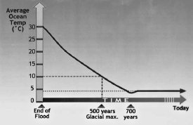
Figure 9.1. Graph of the average temperature of
the ocean following the Flood. The average ocean temperature cooled
below today’s average as the Ice Age glaciers melted because the
atmospheric temperature at higher latitudes was much below the
present. |
I also discovered that the rate of glaciation was controlled by
the amount of volcanic dust and gases in the stratosphere at any one moment. The
more the volcanic effluents, the faster the evaporation and the greater the ice
built up and spread. The less the volcanic debris, the slower the ice built up.
It is conceivable that glaciers retreated a little during volcanic lulls, only
to surge during times of greater volcanism. Variable amounts of volcanism would
have resulted in active ice sheets.
Ice sheet thickness
It may seem impossible to calculate the
thickness of the ice sheets at the peak of the Ice Age, but there is a method
that can be used to provide a ballpark average. It can be done by estimating the
amount of available moisture, the percentage of the precipitation that falls on
the ice sheets, and the length of time to reach glacial maximum. This also has
been developed in more detail elsewhere.2
I will only give the reader the highlights.
There are two main sources of moisture:
(1) evaporation from the warm ocean at mid and high latitudes, and (2)
atmospheric moisture transport from low latitudes. As it turns out, the first
variable is the main source of moisture. Based on maximum and minimum values for
the proportion of the moisture to fall on the ice sheet, I obtained for the
Northern Hemisphere a minimum depth of 1,700 feet (500 m) and a maximum depth of
2,970 feet (900 m). Using variables for the mid range, I estimated an average
depth of 2,300 feet (700 m). The average yearly precipitation over the ice
sheets would have been 55 inches/year (1.4 m/yr). This rate is three times the
current average precipitation over land north of 40°N.3
This is a conservative increase from today considering the huge amount of
evaporation at mid and high latitudes from a warm ocean.
Since nearly all of the ice in the Southern Hemisphere ended up
on Antarctica, I made a similar calculation for the average ice depth on
Antarctica. Interestingly, the best estimate came out to be about 3,900 feet
(1,200 m). The yearly average precipitation in water equivalents would have been
95 inches/year (2.4 m/yr). Antarctica had a thicker ice sheet because of a
greater ocean-to-land distribution. In other words, the Southern Hemisphere
oceans were able to supply more water vapor to storms circling Antarctica.
The above estimates for ice depth are averages. It is expected
that some areas of the ice sheet would be thicker and other areas thinner. The
depth depends upon how close the area was to a main storm track and the amount
of moisture the storm carried. The latter factor is usually related to how close
the storm was to the moisture source — the warm ocean.
The above estimates also assume no summer melting. This is
probably a good assumption for most of the ice sheet, but along the periphery,
some summer melting would be expected. The periphery is a 400-mile (640-km) wide
strip along the edge of the ice sheets. Summer melting would tend to decrease
the ice depth along the edge. However, I never took into account a third
moisture source, and that is the moisture picked up over wet non-glaciated land
in the mid and high latitudes. With possibly three times more precipitation than
today over non-glaciated lands with large lakes occupying currently desert and
semi-arid areas, significant evaporation would have occurred from land. Some of
this evaporation from this third source of moisture would have been added as
snow to the ice sheet. This should mostly compensate for summer melting.
Therefore, neither variable was considered in the ice depth calculations. I
assumed that summer melting and extra snow supplied from evaporation originating
from non-glaciated lands would cancel each other out.
Uniformitarian ice thickness estimates exaggerated
Uniformitarian scientists have claimed
that the ice piled up to over 10,000 feet (3,000 m) thick over eastern Canada
during the Ice Age with an average more like 5,000 feet (1,500 m) (figure 9.2).
The Scandinavian and Cordilleran ice sheets were similarly thought to have been
thick. These ice depths are much thicker than the depths calculated for the
post-Flood model. Which estimate comes closest to the actual depths? First, I
will examine the basis for uniformitarian estimates and then provide data that
indicates that the ice sheets were thinner.4
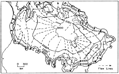
Figure 9.2. This illustration shows the view of
Denton and Hughes of the Laurentide ice sheet of eastern and central
Canada and the Cordilleran ice sheet over British Columbia. |
Uniformitarian geologists mostly have
assumed that the melted ice sheets from the Ice Age were of similar
thickness to those on Greenland and Antarctica. This is part of their “present
processes occurring over millions of years” mindset. They have reasoned that,
given enough time, these past ice sheets should have built up to the size of the
present ones. Arthur Bloom,5 in referring
to the past Laurentide ice sheet, states:
Unfortunately, few facts about its thickness are known. … In
the absence of direct measurements about the Laurentide ice sheet, we must
turn to analogy and theory.
The only analogy or examples we have today are the Greenland and
Antarctica ice sheets. As for theory, uniformitarian scientists assume the ice
developed in the far north of North America and flowed uphill to the southern
periphery after many thousands of years. In this case, the ice at the center, in
Canada, would have to be very thick since glaciers on fairly level terrain flow
from a region of thicker ice to areas of thinner ice. In other words, the
downward slope at the top of the ice sheet determines the glacial motion over
generally level terrain. So, based on both analogy and theory, the
uniformitarian estimate of the ice thickness is quite large, but it is totally
speculative.
Geologists have also used estimates of
sea level lowering to infer ice sheet thickness. However, it is difficult to
determine how low the sea fell during the peak of the Ice Age because the
evidence is underwater. It is interesting that geologists have often estimated
the drop in sea level based on their postulated ice sheet thickness. This
is circular reasoning, since both lower sea level and ice thickness are both
unknown. When it comes right down to it, geologists are really guessing ice
sheet thickness. Ericson and Wollin6
admit: “The estimates vary because one can only guess how thick ice sheets
were.”
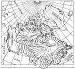
Figure 9.3. The new
multidomed model of the Laurentide ice sheet with two main centers
over Labrador and Keewatin. Arrows are postulated flow paths out
from these domes. There are several other smaller domes postulated,
one of which is shown as the Foxe/Baffin Ice Dome.
View full-size. |
There is some recent evidence, however, that the past ice sheet
thicknesses were significantly lower than uniformitarian scientists expected.
Instead of one big Laurentide ice sheet with a center over Hudson Bay, most
geologists now conclude that there were at least two main ice domes, one east of
Hudson Bay in Labrador and one west and northwest of Hudson Bay, the Keewatin
dome (figure 9.3). This is based mainly on the direction of striated bedrock and
the dispersion of glacial debris. There probably were other ice domes, for
instance the Foxe/Baffin Dome in figure 9.3. Another dome possibility built up
just north of the Great Lakes. Regardless, two or more domes instead of one dome
imply a thinner ice sheet.
Furthermore, the periphery of the
Laurentide ice sheet in the north central United States is now known to have
been much thinner than earlier thought. The original estimates of thicker ice
were based on the thick periphery of the Antarctica ice sheet. The evidence for
a thinner periphery comes from observations that the tops of mountains in north
central Montana, the western Cypress Hills of southeast Alberta, and the Wood
Mountain Plateau in southwest Saskatchewan were all found to be above the ice.7
Ice thickness in southern Alberta and Saskatchewan was rather variable, but was
around 1,000 feet (300 meters) deep. The ice surface slope in southern Alberta
to its southern terminus was nearly flat.8
This thickness is about 1/5 the thickness postulated by using the edge of the
Antarctica ice sheet as an analogy. With such a flat slope and a general uphill
topography from southern Canada into Montana, mainstream scientists are left
with a quandary: how did the ice sheet spread into north central Montana moving
uphill? According to the way glaciers move, it should have been impossible. The
most likely explanation is that the snow and ice had to form generally in place,
as predicted in the post-Flood Ice Age model.
Further evidence for a thin ice sheet
comes from the northern Midwest United States. It is now known that ice lobes
along the margin in this area surged southward. These surges left behind lateral
moraines. The gentle slope of these lateral features indicates that the ice
sheet must have been notably thin.9 The
driftless area in southwest Wisconsin suggests thin ice lobes missed this area
entirely. If the periphery ice were not thin, the driftless area would have been
buried by ice.
Not only was the southwest and
south-central periphery of the Laurentide ice sheet thin, but recent evidence
indicates the northwest margin in the eastern Yukon Territory was also thin.10
The southeast margin in New England was relatively thick. There is little
information from other areas of the periphery of the Laurentide ice sheet.
Occhietti11
sums up the significance of the new observational data:
These results change the concept of the Laurentide ice sheet
radically. They imply, notably, a much smaller ice volume, and complex
margins. http://www.answersingenesis.org/home/area/fit/chapter9.asp
